Quantum Dissipative System

2025 WiSe in Universität Heidelberg · Lecture Notes by Offensive77

This post was translated from Typst to Markdown by Claude Opus 4.8. See the link for the original version.

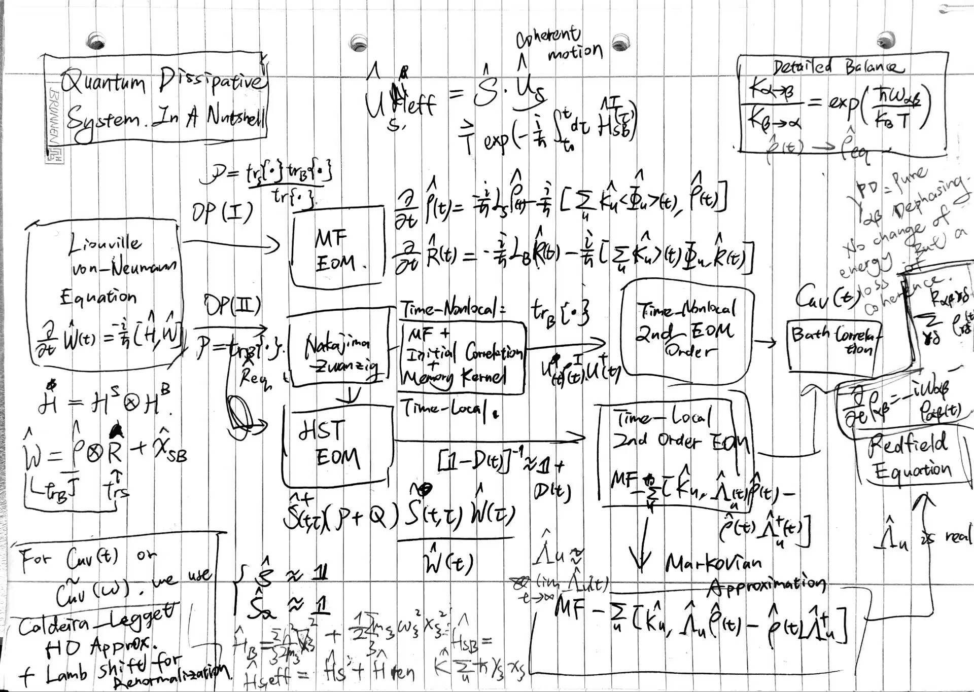
1. Key Tricks Performed in This Topic

1.1. Statistical Operator

Statistical operator (or density operator) reflects the statistical attributes of our system. It works similarly as the probability density function in probability theory. It allows us to define something like expectation and thus correlation.

where $\hat{W}$ is the statistical operator.

Also, for the energy eigenbasis $\{|\alpha ⟩\}$ , we can define the coherence and population of states by:

• Population: $p_{\alpha }(t)=W_{\alpha \alpha }(t)=⟨\alpha |\hat{W}(t)|\alpha ⟩$ ;
• Coherence: $W_{\alpha \beta }(t)=⟨\alpha |\hat{W}(t)|\beta ⟩$ .

Note that:

1.2. Reduced Spaces and Operators

In QDS, we usually separate the system into two parts: what’s relevant and the bath. We are working with the Hilbert space ${\mathcal{H}}_S\otimes {\mathcal{H}}_B$ . Thereby, we write the Hamiltonian as:

or strictly,

where ${\hat{H}}_{SB}=\sum _u{\hat{K}}_u\otimes {\hat{\mathrm{\Phi }}}_u$ is oftentimes used decomposition, which essentially means that ${\hat{H}}_{SB}$ connects the two parts of our system.

We use partial trace to obtain the system and bath reduced statistical operators, which describes the statistical traits of the subsystem.

Notably, a statistical operator can usually not be written as the tensor product of two reduced statistical operators, i.e.

1.3. Schrödinger $\iff$ Interaction Picture

It’s very hard to handle the interaction term ${\hat{H}}_{SB}$ if we stay in the Schrödinger picture. We want a picture where we can get rid of the coherent motion resulted from ${\hat{H}}_S$ and ${\hat{H}}_B$ . The answer is interaction picture:

where ${\hat{H}}_0={\hat{H}}_S+{\hat{H}}_B$ .

Usually, after we obtain some nice results in the interaction picture, we will switch back to Schrödinger picture.

1.4. Orthogonal Projectors

With projectors $\mathcal{P}$ , $\mathcal{Q}$ , we are able to separate the statistical operator into the relevant part and the correlation part.

2. How We Develop the Theory

1. We study the statistical operator, instead of the wave function.
2. We start from the von Neumann equation, instead of the Schrödinger equation, to study the time-evolution of statistical operator.
3. We take the statistical operator as time-dependent. In other words, we choose Schrödinger picture.
4. We insert $\mathcal{P}+\mathcal{Q}=\mathbb{1}$ , whenever needed.

3. First Order Perturbation Theory: Mean Field

Let us study the time-evolution of system operator $\hat{\rho }(t)$ . Define the orthogonal projector $\mathcal{P}$ and $\mathcal{Q}$ into relative system and bath respectively:

We know the time evolution of the full system, by von Neumann EOM:

Apply the partial trace ${\mathrm{tr}}_B$ to Equation (3.2):

Here, ${\mathcal{L}}_B$ term disappears under trace over bath, and we can freely exchange ${\mathrm{tr}}_B$ with ${\mathcal{L}}_S$ . Exploit ${\hat{H}}_{SB}=\sum _u{\hat{K}}_u{\hat{\mathrm{\Phi }}}_u$ :

Insert Equation (1.1) into Equation (3.4):

Define the effective Liouville operator as:

Now, the mean-field approximation arises:

4. Beyond MF: Travel to Interaction Picture

This is only a rough estimation, which is unitary, meaning that it conserves energy (no dissipation at all). Even worse, if the bath is in thermal equilibrium, the time-dependent unitary evolution will devolve into a simple unitary evolution:

Assume the bath is in thermal equilibrium, which means its statistical operator reads

and it is not subject to the changes of our relevant system. Define a new set of orthogonal projectors:

In this part, we try to derive time-evolution in the interaction picture, and travel back to Schrödinger picture afterwards.

4.1. Nakajima–Zwanzig Equation

We can write the similar thing for $\mathcal{Q}{\hat{W}}_I(t)$ :

Can we exactly solve for $\mathcal{Q}{\hat{W}}_I(t)$ ? Yes. Solve the homogeneous part, then make ansatz for the inhomogeneous solution, and solve again. The NZ equation is obtained from such way as:

Analysis of NZ equation:

• $\mathcal{P}{\mathcal{L}}_{SB}^I(t)\mathcal{P}{\hat{W}}_I(t)$ : Exactly mean field;
• $\mathcal{P}{\mathcal{L}}_{SB}^I(t){\mathcal{S}}_{\mathcal{Q}}(t,t_0)\mathcal{Q}{\hat{W}}_I(t_0)$ : Initial system-bath correlation $(\mathcal{Q}{\hat{W}}_I(t_0))$ , after some evolution, coming back to affect the relevant systems again;
• ${\int }_{t_0}^t\mathrm{d}\tau \mathcal{P}{\mathcal{L}}_{SB}^I(t){\mathcal{S}}_{\mathcal{Q}}(t,\tau )\mathcal{Q}{\mathcal{L}}_{SB}^I(\tau )\mathcal{P}{\hat{W}}_I(\tau )$ : Memory kernel over the full time interval.

4.2. HST Equation

By insert into the solution of $\mathcal{Q}{\hat{W}}_I(t)$ the equation below:

we can put the integral into a new super operator and get rid of the time-nonlocality of the NZ equation.

5. Exploit NZ Equation

5.1. Time-Nonlocal Second-Order EOM

Taking the trace over bath on the NZ equation leads to:

In practice, we usually assume the initial correlation to be zero. And we approximate ${\mathcal{S}}_{\mathcal{Q}}(t,\tau )$ by the first order Taylor expansion, in other words, $\mathbb{1}$ . The equation then reads:

To further evaluate the equation, we need to insert $\mathcal{Q}=\mathbb{1}-\mathcal{P}$ , then perform ${\mathcal{L}}_{SB}^I(t)$ twice, which leads to 8 terms. Final result:

Note that one can re-write this equation by defining an effective Liouville super-operator that includes the system Liouville operator and the mean-field contributions and an integral kernel as

Eq. (7.2.52) is typically the one implemented within a numerical simulation after the bath correlation functions have been obtained. Our bath correlation function is given by:

It describes the correlation inside the bath. And it will act back to our relevant system by the system operator $\hat{K}$ 's.

5.2. Obtain Bath Correlation Function

In practice, it’s hard to obtain the bath correlation function $C_{uv}(t)$ directly. However, ${\tilde{C}}_{uv}^{-}(\omega )$ in the Fourier domain, can be computed by experiments.

Afterwards, we can apply an inverse Fourier Transform to our obtained ${\tilde{C}}_{uv}^{-}(\omega )$ :

6. Analyze the Bath

6.1. Linear Response

Assume the bath is in the thermal equilibrium at $t_0$ . Recall the MF EOM of the bath:

Come to interaction picture by write:

where ${\hat{S}}_{\mathrm{Int}}(t,t_0)=\hat{\mathcal{T}}\exp (-\frac{i}{\hslash }{\int }_{t_0}^t\mathrm{d}\tau \sum _u{\hat{\mathrm{\Phi }}}_u⟨{\hat{K}}_u⟩(\tau ))$ . Approximate ${\hat{S}}_{\mathrm{Int}}$ by second-order Taylor expansion:

and assume ${\hat{\mathrm{\Phi }}}_u$ and ${\hat{K}}_u$ are Hermitian. The expectation value of ${\hat{\mathrm{\Phi }}}_u$ is now time-dependent:

where ${\chi }_{uv}(t)=-i\hslash C_{uv}^{-}(t)$ is called linear response or linear susceptibility. It, same as bath correlation function, describes the internal reorganization of the bath.

6.2. Fluctuation–Dissipation Theorem

We study now the dissipation of bath energy:

Note that the trace over commutators gives 0. The fluctuation around thermal equilibrium, described by $\chi$ , decides the dissipation of energy itself.

7. Caldeira–Leggett Approximation for Bath

This chapter contains some artificial things to oversimplify our bath.

7.1. Bath as Harmonic Oscillators

The idea is assuming the bath to be a set of Harmonic Oscillator, to obtain our bath correlation easily:

And Taylor expand the bath part of ${\hat{H}}_{SB}$ to the first order:

We then can express the coordinate in creation/annihilation operators:

where $g_{\xi }={\gamma }_{\xi }\sqrt{{\displaystyle \frac{\hslash }{2m_{\xi }{\omega }_{\xi }^3}}}$ . Then, we can write the bath correlation function:

After a lot of math:

7.2. Spectral Density Function

To introduce a more compact form of our bath correlation function, we use:

Then,

Furthermore, by $n(-\omega )=-(1+n(\omega ))$ , there holds

The spectral density function encodes the strength of absorption at frequency $\omega$ . If the bath states are dense, we can naturally choose continuous spectral density function.

7.3. Lamb Shift

We may notice that $⟨\hat{\mathrm{\Phi }}⟩=0$ for our assumed $\hat{\mathrm{\Phi }}=\sum _{\xi }\hslash {\gamma }_{\xi }{x}_{\xi }$ , this is however often not the case. To mend it we must introduce a renormalization Hamiltonian to our system Hamiltonian.

The derivation is by equating $\partial \hat{H}/\partial x_{\xi }$ to zero.

8. Exploit HST

8.1. Time-Local Second Order EOM

The difficulty in handling the HST equation is the inverse of super operator. However, we can perform the Taylor expansion on it to simplify that:

Do the similar thing we did for the NZ equation as in Section 5.1, we obtain:

where ${\hat{\mathrm{\Lambda }}}_u(t)=\sum _v{\int }_{t_0}^t\mathrm{d}\tau C_{uv}(t-\tau ){\hat{K}}_v^I(\tau -t)$ .

8.2. Markovian Approximation

The idea is, since $C_{uv}(t)$ vanishes after a short time, we can approximate the ${\hat{\mathrm{\Lambda }}}_u(t)$ as a constant with

Equation (8.2) becomes now

8.3. Redfield Equation

We skip the technical derivations and just look at the obtained EOM, represented in eigenstates of system Hamiltonian ${\hat{H}}_S$ .

$R$ is called Redfield Tensor. Recall that the diagonal elements of density operator ${\rho }_{\alpha \alpha }$ are called the population of state $\alpha$ , and the off-diagonal elements ${\rho }_{\alpha \beta }$ are called the coherence. We study now how Redfield tensor affects our reduced density operator.

8.3.1. $R_{\alpha \alpha \gamma \gamma }$

This component describes the change of population of state $\alpha$ is made of the transfer from $\alpha$ to all other states $\epsilon$ and from other state $\gamma$ to $\alpha$ .

8.3.2. $R_{\alpha \beta \alpha \beta }$

This component describes the change of coherence between state $\alpha$ and $\beta$ is made of the transfer from both $\alpha$ and $\beta$ to all other states $\epsilon$ , and the pure dephasing ${\gamma }_{\alpha \beta }^{\mathrm{PD}}:=-{\mathrm{\Gamma }}_{\alpha \alpha \beta \beta }-{\mathrm{\Gamma }}_{\beta \beta \alpha \alpha }$ .

8.3.3. Exponential Decay of Population

Population life-time is given by:

Meanwhile, the coherence life-time is:

8.4. Detailed Balance

By looking at again the transfer rate, we obtain

It ensures that the relevant system reaches thermal equilibrium at long times because there is a thermal weight factor between rates connecting states of different energy. The system will assume a dynamic equilibrium between excitation and de-excitation mediated by the thermal heat bath. Assume that the energy of state $\alpha$ is higher than $\beta$ . Then ${\omega }_{\alpha \beta }=(E_{\alpha }-E_{\beta })/h>0$ . We have that transition from $\alpha$ to $\beta$ happens more frequently than from $\beta$ to $\alpha$ .