From Maxwell's Fluid to Oldroyd-B (II): Objective Derivatives
Non-Newtonian Fluid Seminar 01 · Universität Heidelberg
This post is the second part of the script of my seminar talk From Maxwell’s Fluid to the Oldroyd-B Model, translated from Typst to Markdown. The series:
In the last post we saw that the tensorial Maxwell model
fails: the material derivative
is not frame invariant, so different observers see different dynamics. We need a time derivative that every observer agrees on.
1. A Boat Ride to Objective Derivatives
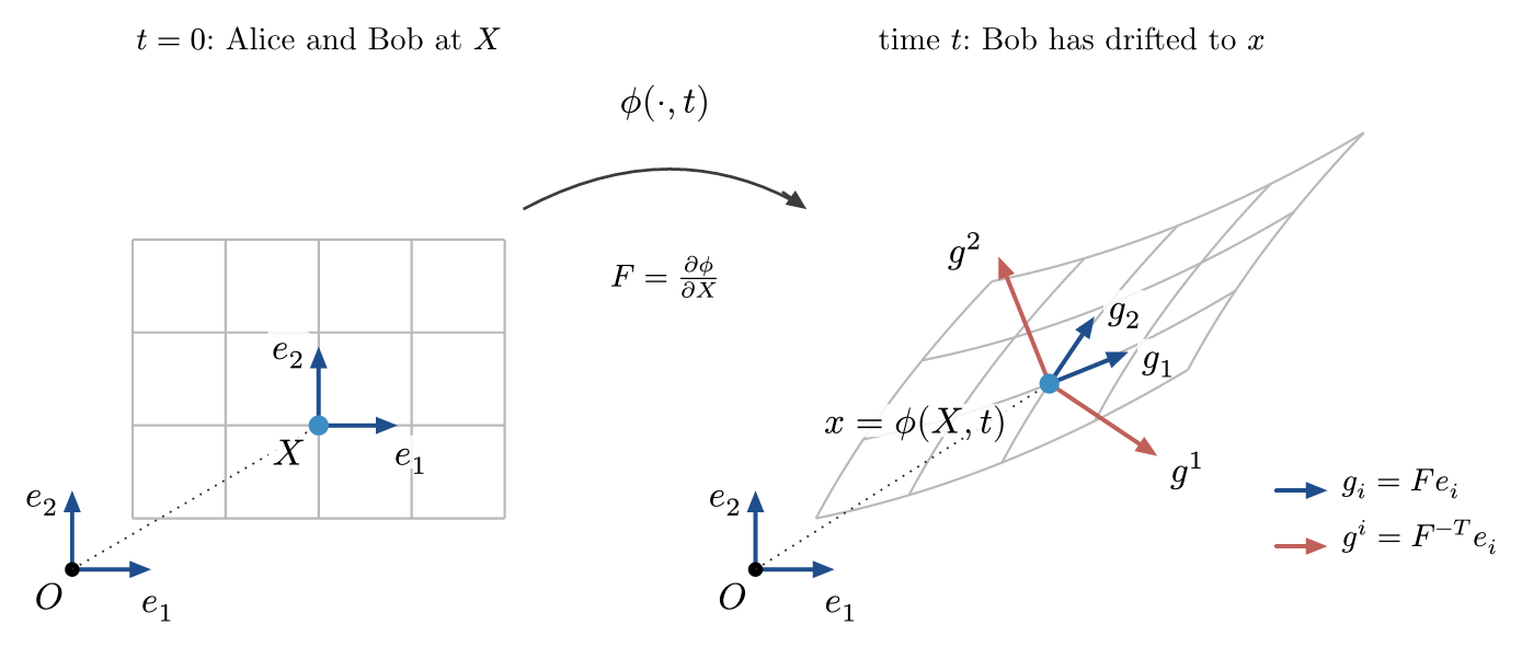
For the introduction to objective derivatives, let’s take a boat ride. At time
, Alice and Bob stand in a laboratory on a lake, at the point
. They want to observe some quantity
. To them, a tensor such as
is a magical black box: it eats two vectors and spits out a number. Their only tools are the arrows of an orthonormal Cartesian basis
, painted on the surface of the water. To measure
, they feed it the pair
and record
This is the observation of
in
.
Then Bob goes for a boat ride. He does not row; he simply drifts with the water. After a time
he arrives at
(Figure 1). The arrows painted on the water have drifted with him, but the flowing lake has stretched and sheared them into
which are no longer orthonormal. To read off components with such arrows, Bob also needs the dual basis
, defined by
.
Figure 1. Left: the basis eᵢ painted on the water at X. Right: after drifting to x, Bob finds the arrows carried and deformed by the flow, gᵢ = F eᵢ (blue), together with their dual basis gⁱ = F⁻ᵀ eᵢ (red), which is normal to the deformed material lines.
2. Push-Forward and Pull-Back
To Bob, the quantity now looks like a different tensor
, although it is essentially the same thing. Bob therefore insists that the observation be preserved: measured with his deformed arrows,
must give the same numbers that
gave Alice,
Writing
and moving
into the ket,
Comparing with Alice’s observation, Bob finds
.
Push-Forward and Pull-Back
The map
is called the push-forward, and
the pull-back.
Since
is exactly how line elements are carried by the flow, this form tells us that
changes the way line elements do, just like a polymer chain stretched by the flow.
3. Upper-Convected Derivative
Now Bob wants to know how fast
changes. His idea is simple: go back to the one fixed frame he shares with Alice. He pulls
back to
in
, takes the time derivative there, and pushes the result forward. With the velocity gradient
, the material derivative
, and
,
, this gives the upper-convected derivative:
Upper-Convected Derivative (UCD)
In short: pull back, differentiate, push forward. The UCD measures change relative to the flow.
4. Lower-Convected Derivative
With different choices of the push-forward and pull-back, we can define other objective derivatives. For example, the lower-convected derivative is defined by
Lower-Convected Derivative (LCD)
The same story produces it. Suppose Bob had measured with the carried arrows
instead of the dual ones, and insisted on
. Since
, he would find
. Pulling back, differentiating with
, and pushing forward gives
UCD vs. LCD
The dual arrows are normal to the deformed material lines, so the LCD carries like normals of material surfaces, while the UCD carries it like line elements. A polymer chain is a line element; this is the microscopic reason for choosing the UCD.
With the UCD at hand, we are ready to repair the Maxwell model in the next post.